Gradient Calculation
In the last few videos, we learned that in order to minimize the error function, we need to take some derivatives. So let's get our hands dirty and actually compute the derivative of the error function. The first thing to notice is that the sigmoid function has a really nice derivative. Namely,
\sigma'(x) = \sigma(x) (1-\sigma(x))σ′(x)=σ(x)(1−σ(x))
The reason for this is the following, we can calculate it using the quotient formula:
And now, let's recall that if we havemmpoints labelledx^{(1)}, x^{(2)}, \ldots, x^{(m)},x(1),x(2),…,x(m),the error formula is:
E = -\frac{1}{m} \sum_{i=1}^m \left( y_i \ln(\hat{y_i}) + (1-y_i) \ln (1-\hat{y_i}) \right)E=−m1∑i=1m(yiln(yi^)+(1−yi)ln(1−yi^))
where the prediction is given by\hat{y_i} = \sigma(Wx^{(i)} + b).yi^=σ(Wx(i)+b).
Our goal is to calculate the gradient ofE,E,at a pointx = (x_1, \ldots, x_n),x=(x1,…,xn),given by the partial derivatives
\nabla E =\left(\frac{\partial}{\partial w_1}E, \cdots, \frac{\partial}{\partial w_n}E, \frac{\partial}{\partial b}E \right)∇E=(∂w1∂E,⋯,∂wn∂E,∂b∂E)
To simplify our calculations, we'll actually think of the error that each point produces, and calculate the derivative of this error. The total error, then, is the average of the errors at all the points. The error produced by each point is, simply,
E = - y \ln(\hat{y}) - (1-y) \ln (1-\hat{y})E=−yln(y^)−(1−y)ln(1−y^)
In order to calculate the derivative of this error with respect to the weights, we'll first calculate\frac{\partial}{\partial w_j} \hat{y}.∂wj∂y^.Recall that\hat{y} = \sigma(Wx+b),y^=σ(Wx+b),so:
The last equality is because the only term in the sum which is not a constant with respect tow_jwjis preciselyw_j x_j,wjxj,which clearly has derivativex_j.xj.
Now, we can go ahead and calculate the derivative of the errorEEat a pointx,x,with respect to the weightw_j.wj.
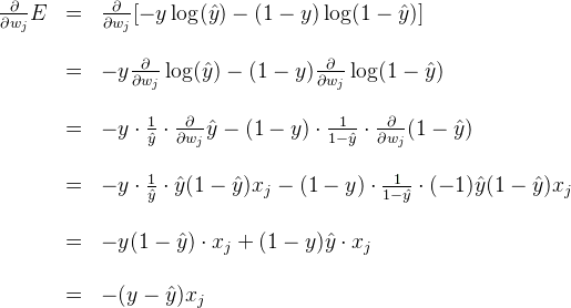
A similar calculation will show us that
This actually tells us something very important. For a point with coordinates(x_1, \ldots, x_n),(x1,…,xn),labely,y,and prediction\hat{y},y^,the gradient of the error function at that point is\left(-(y - \hat{y})x_1, \cdots, -(y - \hat{y})x_n, -(y - \hat{y}) \right).(−(y−y^)x1,⋯,−(y−y^)xn,−(y−y^)).In summary, the gradient is
\nabla E = -(y - \hat{y}) (x_1, \ldots, x_n, 1).∇E=−(y−y^)(x1,…,xn,1).
If you think about it, this is fascinating. The gradient is actually a scalar times the coordinates of the point! And what is the scalar? Nothing less than a multiple of the difference between the label and the prediction. What significance does this have?
퀴즈 질문
What does the scalar we obtained above signify?
Closer the label to the prediction, larger the gradient.
Closer the label to the prediction, smaller the gradient.
Farther the label from the prediction, larger the gradient.
Farther the label to the prediction, smaller the gradient.
제출
So, a small gradient means we'll change our coordinates by a little bit, and a large gradient means we'll change our coordinates by a lot.
If this sounds anything like the perceptron algorithm, this is no coincidence! We'll see it in a bit.
Gradient Descent Step
Therefore, since the gradient descent step simply consists in subtracting a multiple of the gradient of the error function at every point, then this updates the weights in the following way:
w_i' \leftarrow w_i -\alpha [-(y - \hat{y}) x_i],wi′←wi−α[−(y−y^)xi],
which is equivalent to
w_i' \leftarrow w_i + \alpha (y - \hat{y}) x_i.wi′←wi+α(y−y^)xi.
Similarly, it updates the bias in the following way:
b' \leftarrow b + \alpha (y - \hat{y}),b′←b+α(y−y^),
_Note:_Since we've taken the average of the errors, the term we are adding should be\frac{1}{m} \cdot \alpham1⋅αinstead of\alpha,α,but as\alphaαis a constant, then in order to simplify calculations, we'll just take\frac{1}{m} \cdot \alpham1⋅αto be our learning rate, and abuse the notation by just calling it\alpha.α.